The newsvendor model revisited: the impacts of high unit holding costs on the accuracy of the classic model

Abstract

The newsvendor problem has been applied in various business settings. It is often assumed that the decision variable, i.e., order-up-to level, has no impacts on the holding costs for average inventory cycled in a given period, which is the difference between beginning and ending inventory levels on hand in that period. The average holding cost for this portion of inventory is conveniently and approximately calculated as half the product of the unit holding cost and the expectation of the demand in one period if it is assumed that the inventory is approximately evenly consumed. It is a good approximation when the unit holding cost is significantly lower than the unit backorder cost as this optimal solution to inventory level is able to guarantee a low probability of understocking. However, if this condition does not hold, the approximation may deviate from the actual cost and cannot measure the expected holding cost for this portion of inventory. This paper examines the impact of the cycle stock holding cost on the newsvendor model and the conditions under which this portion of cost is not negligible.

Introduction

The newsvendor model is fundamental for stochastic inventory management theories, which has been studied and applied in various business settings (e.g., Erlebacher, 2000; Mieghem, 2007; Olivares et al., 2008; Petruzzi et al., 2009; Krishnan et al., 2010). Consider a typical single period newsvendor model. An optimal inventory level is determined to minimize the expected cost, usually including the ordering cost, and the expected overstocking and shortage costs. Ordering too many items can incur overstocking costs, while ordering too few can cause shortage costs. In this typical model, it is often assumed that the decision variable, i.e., order-up-to level, has no impacts on the holding cost for the average inventory consumed in a specific period, which is the difference between beginning and ending inventory levels at hand in that period. Consumed stocks are items that are sold or used by the holder in a particular period. In the classic model, the average holding cost for this portion of inventory is conveniently and approximately calculated as half the product of the unit holding cost and the expectation of the demand in that period, if it is assumed that the inventory is approximately evenly consumed. It is a good approximation when the unit holding cost is much lower than the unit shortage cost because the optimal inventory level of the classic newsvendor model can lessen the possibility of understocking. However, if this condition does not hold, the approximation may deviate from the actual cost and cannot measure the expected holding cost for this portion of inventory accurately. In fact, the unit holding cost for certain products may experience a quick increase. Factors that determine the unit inventory holding cost usually include storage space costs, handling and service costs, risk costs and capital costs. One or more of the above factors may lead to a high unit holding cost. For example, luxury products usually have a high capital cost due to their high ordering costs, and a high risk cost for insurance. Goods that require specific storage conditions, e.g., isoperibol, refrigeration, temporary control or air conditioning may also incur a high unit holding cost. For instance, in Qingdao, a city in North China which is well-known as a seafood distribution center, the rent for cold warehouses for seafood has continuously increased for the past two years. This is mainly because cold storage units are being charged heavily for pollution violations by the local Environmental Protection Bureau. With the ratification of the Paris Climate Agreement in 2015, many countries have committed to cutting greenhouse gas emissions significantly by 2030. Carbon charging has been implemented in several pilot markets in China including Qingdao and will be implemented nation-wide in the near future. Prices for CO₂ emitted by energy consumption for storage are likely to continue its increase as a way to address global warming. Indeed, such pricing has already been in effect in a number of industries in the European Union for many years. These kinds of policies push up the unit holding cost for storage, which in turn affects the accuracy of the traditional newsvendor model. Other factors can also drive up holding costs. In modern warehouses armed with advanced technologies, to smooth the process, many goods are labeled with RFID tags. As is well-known, RFID can greatly enhance the efficiency and effectiveness of warehouse management, although it incurs much higher costs compared to traditional bar coding systems. Overall, holding costs have been experiencing a sharp increase recently in some specific industries.

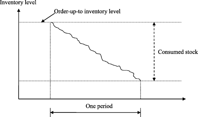
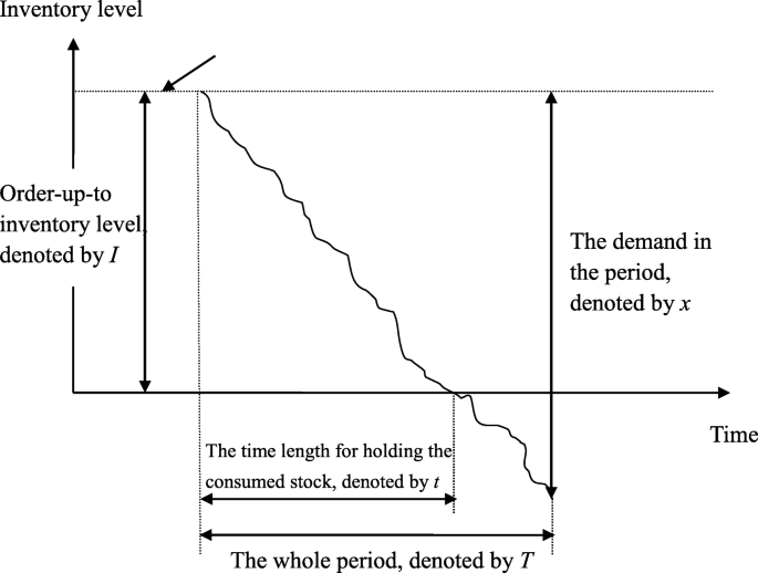
To examine the inaccuracy of the classic newsvendor model when the unit holding cost is high, we analyze two scenarios with different inventory levels at the end of one period in Figs. 1 and 2. Figure 1 shows the scenario where overstocking occurs at the end of the period, and the consumed inventory used to meet customers’ demand is the difference between the beginning and ending inventory levels. In contrast, Fig. 2 shows the scenario where understocking takes place at the end of the period, the consumed inventory equals the beginning inventory level and there is unsatisfied demand at the end of the period. The unit holding cost is defined as the cost for one item held in the warehouse for the whole period. In the first scenario (Fig. 1), all demand in the period is satisfied, and the average consumed inventory approximately equals half the demand if it is assumed that the inventory is approximately evenly consumed. The approximation works well herein. In contrast, in the second scenario (Fig. 2) with unsatisfied demand, inventory has been used up before the end of the period. Then it is not appropriate to take half the demand as the approximation of the average consumed inventory. In this scenario the approximation is not very accurate and the degree of deviation greatly depends on the critical ratio of the newsvendor model. We can also observe that the decision variable, i.e., order-up-to level, does influence the holding cost for consumed inventory.

Fig. 1

The situation where overstock occurs at the end of one period

Fig. 2

The situation where out-of-stock occurs at the end of one period (with notation)

In the literature, most prior research has not considered the holding cost for consumed inventory in the cost (objective) function and has employed the approximation. There are two possible reasons. First, if the unit holding cost is much lower than the unit shortage cost, the optimal inventory level that is derived from the cost function considering ordering, overstocking and shortage costs can lessen the possibility of understocking, and the approximation is an accurate one to measure the holding cost for consumed goods. In this situation, whether this portion of the holding cost is added to the cost function does not affect the optimal inventory level much. A detailed explanation is also shown in the numerical experiment of this paper. Second, the newsvendor model, without considering the holding cost for consumed goods, can provide a compactly analytic solution, which is convenient for further analysis such as multi-echelon problems and multi-tier supply chain problems. For many cases where the ratio of unit holding cost to unit shortage cost is low, the approximation is accurate and skipping the holding cost for consumed inventory in the cost function is acceptable. However, when the unit holding cost is not much lower or even higher than the unit shortage cost, it may cause a non-ignorable deviation from the actual optimal inventory level that minimizes the sum of the expected ordering cost, shortage cost and holding cost for consumed and overstocked items. In such cases, we cannot ignore the consumed inventory holding cost in the cost function for simplification and should seriously consider it when we determine the optimal inventory level.

The rest of this paper is organized as follows. Section “Literature Review” reviews the related literature on newsvendor models. In Section “Newsvendor Models with Consumed Inventory Holding Cost”, the model that includes the consumed inventory holding cost is constructed and analyzed. In Section “Numerical Experiments”, numerical experiments are conducted to analyze the cases where the holding cost for consumed inventory becomes non-ignorable. Section “Conclusion” concludes the whole paper and extends the discussion.

Literature review

The newsvendor model is one of the fundamental models for Operations Research and Management Science. Porteus (1990) summarizes the typical newsvendor model for one-period and multi-period cases. The ordering cost, and overstocking and understocking costs are considered in the cost function and the unsatisfied demand at the end of one period is either lost or backlogged. The critical ratio that is the optimal probability of not stocking out is the ratio of the unit underage cost to the sum of the unit underage and overage costs. Arrow et al. (1951) give the first derivation of the optimal inventory level and reorder point as a function of the demand distribution, the cost of making an order, and the overstocking and understocking costs. Arrow and Karlin (1958a,1958b) analyze the optimality of the base stock policy for one stage inventory models with uncertain demand. The optimal inventory level can be determined by examining the derivative of the objective function. Concerning the batch ordering problem of the newsvendor model, Veinott (1965a) shows that a base stock policy, with which the stock is replenished to a certain level if possible, is still optimal. For a single period model with convex objective function and setup cost for ordering, an (s, S) policy is optimal. Karlin (1958a) and Porteus (1971, 1972) examine the conditions under which a generalized (s, S) policy is optimal. Porteus (1971, 1972) and Heyman and Sobel (1984) further show that an (s, S) policy will still be optimal if the objective function is a quasi-K-convex for some K that is less than the fixed ordering cost. Hadley and Whitin (1963) consider the newsvendor model with a single linear constraint on the initial inventory levels for multiple products. Evans (1967) analyzes a newsvendor model with a linear constraint on the total order and shows that the optimal policy is a base stock policy. Veinott (1965b) examines the optimal policy for the multi-period problem and shows that a myopic base stock policy is optimal under a set of conditions and can be found as a solution to the single period newsvendor model with modified unit overstocking and understocking costs. Li and Lin (2006) examine the affecting factors for information sharing and information quality in supply chain management. Ferguson et al. (2007) analyze an extension of the economic order quantity model where the cumulative holding cost is a nonlinear function of time. Berling (2008) examines the problem with a stochastic holding cost. He considers a single-item inventory model with a fixed set-up cost and stochastic purchase price, and assumes the holding cost is the product of interest rates and purchase price. Shi and Yan (2017) analyze features of the heterogeneity of consumer preferences and address the multiple equilibrium of retail formats. In sum, prior research has analyzed the optimal solutions of the basic newsvendor model and has provided extensions that consider the setup cost, batch ordering, linear constraints on the total order and initial inventory levels for multi-product cases, etc. The ordering cost, overstocking and understocking costs are considered in the cost function. To our knowledge, no research addresses the consumed inventory holding cost in the objective function and its impact on the optimal inventory level, while this portion of holding costs does occur. This research aims to narrow this gap. Correia et al. (2013) develop performance measures for a multi-period, two-echelon supply chain network.

Newsvendor models with consumed inventory holding cost

The newsvendor model with instantaneous receipt

In this section, we first formulate the newsvendor model with instantaneous receipt by considering inventory holding costs for consumed inventory in the cost function. At the beginning of the period, an order-up-to inventory level is determined to minimize the sum of the expected cost. At the end of the period, there are two possible scenarios: overstocking or understocking. Figures 1 and 2 show the changes in inventory level when overstocking or understocking occurs respectively. The unsatisfied demand is backlogged if there is understocking. The stocking out cost is the backordering cost. The inventory level determined at the beginning of the period affects the overstocking and understocking costs, as well as the holding cost for consumed inventory during the period. The model is described by the following parameters and variables:

h the unit inventory holding cost;

π the unit backordering cost if shortage occurs;

x the random demand in the period, which follows a normal distribution;

μ the mean of the demand distribution in the period;

σ the standard deviation of the demand distribution in the period;

I the order-up-to inventory level at the beginning of the period;

C(I) the inventory cost when the order-up-to level is I;

φ(•) the probability density function of the demand in the period;

Φ(•) the standard normal distribution function;

E(•) the expected value of a random variable.

Then the objective function of the newsvendor model with instantaneous receipt is

$$ {\displaystyle \begin{array}{l}\underset{I\ge 0}{\min}\kern0.5em C(I)=\pi {\int}_I^{+\infty}\left(x-I\right)\varphi (x)\ dx+h{\int}_0^I\left(I-x\right)\varphi (x)\ dx\\ {}\kern4.5em +\frac{h}{2}{\int}_0^Ix\ \varphi (x)\ dx+\frac{h}{2}{\int}_I^{+\infty}\frac{I^2}{x}\kern0.5em \varphi (x)\ dx.\end{array}} $$

(P1)

The first and second terms in the objective function represent the expected overstocking and understocking costs. The third term is the expected inventory holding cost for consumed inventory if there are items left at the end of the period. This situation is also shown in Fig. 1. The fourth term is the expected consumed inventory holding cost if out-of-stock occurs, which can be derived from the plane-geometry as follows. In Fig. 2, it can be shown that the holding cost for consumed stock is

$$ {\int}_I^{+\infty}\frac{I}{2}\cdot \left(\frac{t}{T}h\right)\varphi (x) dx $$

We can show that $\frac{t}{T}=\frac{I}{x}$ Then we have

$$ {\int}_I^{+\infty}\frac{I}{2}\cdot \left(\frac{t}{T}h\right)\varphi (x) dx=\frac{h}{2}{\int}_I^{+\infty}\frac{I^2}{x}\varphi (x) dx $$

By rearranging Program P1, we get

$$ {\displaystyle \begin{array}{l}\underset{I\ge 0}{\min}\kern0.5em C(I)=\pi \left[E(x)-I\right]+\left(h+\pi \right){\int}_0^I\left(I-x\right)\varphi (x)\ dx\\ {}\kern2.75em +\frac{h}{2}E(x)+\frac{h}{2}{\int}_I^{+\infty}\left(\frac{I^2}{x}-x\ \right)\ \varphi (x)\ dx.\end{array}} $$

(P2)

The sum of the first three terms in Program P2 is the total inventory cost if we use half the product of the unit holding cost and the expectation of the demand in the period to approximate the consumed inventory holding cost, which is usually used in classic newsvendor models. With this approximation, the decision variable I affects the first two terms (i.e., overstocking and understocking costs), but has no impact on the third term, and the optimal inventory level is determined by minimizing the sum of the first two terms, and can be expressed as.

$$ {I}^{\ast \prime }=\mu +{\Phi}^{-1}\left(\frac{\pi }{\pi +h}\right)\sigma $$

(3.1)

However, when we consider the consumed inventory cost in a more accurate way, there is another term $h{\int}_I^{+\infty}\left({I}^2/x-x\ \right)\ \varphi (x)\ dx/2$ in the cost function, which is also affected by the decision variable I. Then the optimal inventory level for Program P2 is different with the one given in (3.1). We take the first-order and second-order derivatives of the objective function with respect to I in Program P2, and we have.

$$ {C}^{\prime }(I)=-\pi +\left(h+\pi \right){\int}_0^I\varphi (x)\ dx+ hI{\int}_I^{+\infty}\frac{1}{x}\varphi (x)\ dx $$

(3.2)

$$ {C}^{{\prime\prime} }(I)=\pi \varphi (I)+h{\int}_I^{+\infty}\frac{1}{x}\varphi (x)\ dx $$

(3.3)

(3.3) shows that the second-order derivative is greater than 0, and therefore the objective function is convex. It should be noted that, due to the second and third terms of the first-order derivative in (3.2), a closed form solution cannot be derived. Denote the solution of C^′(I) = 0 by I^∗, which is the optimal inventory level of Program P2. From (3.2) and (3.3), we can obtain the following theorems.

Theorem 1 The optimal solution to P2, i.e., I^∗, is less than I^∗′ in (3.1).

Proof: We need to prove I^∗′ > I^∗. Substituting I^∗′ into (3.2), we have.

${C}^{\prime}\left({I}^{\ast \prime}\right)={hI}^{\ast \prime }{\int}_{I^{\ast \prime}}^{+\infty}\frac{1}{x}\varphi (x)\ dx$ as $-\pi +\left(h+\pi \right){\int}_0^{I^{\ast \prime }}\varphi (x)\ dx=0$.

Noting ${C}^{\prime}\left({I}^{\ast \prime}\right)={hI}^{\ast \prime }{\int}_{I^{\ast \prime}}^{+\infty}\frac{1}{x}\varphi (x)\ dx>0$, C^′(I^∗) = 0 and C(•) is convex, we can obtain.

I^∗′ > I^∗.

In words, for a single-period newsvendor model, when the expected overstocking and shortage costs at the end of the period and the consumed inventory cost are considered in the cost function, the optimal inventory level for this cost function decided at the beginning of the period is lower than the optimal solution that only minimizes the sum of the expected overstocking and shortage costs at the end of the period.

Theorem 2 The optimal solution to P2, i.e., I^∗, is a decreasing function of the unit holding cost h.

Proof: From (3.2), we obtain

$$ -\pi +\left(h+\pi \right){\int}_0^{I^{\ast }}\varphi (x)\ dx+{hI}^{\ast }{\int}_{I^{\ast}}^{+\infty}\frac{1}{x}\varphi (x)\ dx=0 $$

From this implicit function, we can show

$$ \frac{dI^{\ast }}{dh}=-\frac{\int_0^{I^{\ast }}\varphi (x)\ dx+{I}^{\ast }{\int}_{I^{\ast}}^{+\infty}\frac{1}{x}\varphi (x)\ dx}{\pi \varphi \left({I}^{\ast}\right)+h{\int}_{I^{\ast}}^{+\infty}\frac{1}{x}\varphi (x)\ dx} $$

Then the optimal inventory level I^∗ for this cost function decreases with the unit holding cost.

Theorem 3 The optimal solution to P2, i.e., I^∗, is an increasing function of the unit backordering cost π.

Proof: From (3.2), we obtain

$$ -\pi +\left(h+\pi \right){\int}_0^{I^{\ast }}\varphi (x)\ dx+{hI}^{\ast }{\int}_{I^{\ast}}^{+\infty}\frac{1}{x}\varphi (x)\ dx=0 $$

From this implicit function, we can show

$$ \frac{{d I}^{\ast }}{d\pi}=\frac{1-{\int}_0^{I^{\ast }}\varphi (x)\ dx}{\pi \varphi \left({I}^{\ast}\right)+h{\int}_{I^{\ast}}^{+\infty}\frac{1}{x}\varphi (x)\ dx} $$

Then the optimal inventory level I^∗ for this cost function increases as the unit backordering cost.

In section “Numerical Experiments”, we conduct the numerical experiments to get I^∗, and the expected average inventory cost per period C(I^∗), then compare it withC(I^∗′).

The newsvendor model without instantaneous receipt

In this section, we further consider the newsvendor model without instantaneous receipt for an infinite planning horizon. The demand in each period follows a normal distribution with mean μ and variance σ². Suppose there is a delay of L periods between ordering goods and receiving them. At the beginning of each period, goods ordered L periods ago arrive. During the whole period, the on-hand inventory is consumed approximately evenly to meet customers’ demands, and the unsatisfied demand is backlogged if stocking out occurs. Demands are independent over time. The order-up-to level I _m is determined at the end of the period. We still let h and π denote the unit holding and shortage cost per period, and use the following parameters to formulate the model:

D₁ the demand in one period;

D _L the sum of demand in L periods;

D_L + 1 the sum of demand in L + 1 periods;

φ₁(•) the probability density function of the demand in one period;

φ _L (•) the probability density function of the demand in L periods;

φ_L + 1(•) the probability density function of the demand in L + 1 periods;

I _m the order-up-to level in one period;

C _m (I _m ) the expected average inventory cost when the order-up-to level is I _m .

Then the newsvendor problem without instantaneous receipt can be modeled as

$$ {\displaystyle \begin{array}{l}\underset{I_m\ge 0}{\min }\ {C}_m\left({I}_m\right)=\pi {\int}_{I_m}^{+\infty}\left(x-{I}_m\right){\varphi}_{L+1}(x)\ dx+h{\int}_0^{I_m}\left({I}_m-x\right){\varphi}_{L+1}(x)\ dx\\ {}\kern2.75em +\frac{h}{2}{\int}_0^{I_m}{\int}_0^{I_m-x}x\ {\varphi}_1(x){\varphi}_L(y) dy\ dx\\ {}\kern2.75em +\frac{h}{2}{\int}_0^{+\infty }{\int}_{\max \left(0,{I}_m-x\right)}^{I_m}\left[1-\frac{y+x-{I}_m}{x}\right]\ \left[x-\left(y+x-{I}_m\right)\right]\ {\varphi}_1(x){\varphi}_L(y) dy\ dx.\end{array}} $$

(P3)

In Program P3, the objective function is the expected average inventory cost including overstocking costs, shortage costs and consumed inventory holding costs. Similar to Program P1, the first two terms are the expected overstocking and shortage costs. The third term is the expected inventory holding cost for consumed inventory if there are items left at the end of the period. The last term is a little complicated, which represents the expected holding cost for consumed inventory if there is unsatisfied and backlogged demand in the period. The value of this term is determined by the on-hand inventory level at the beginning of the period that is the difference between the order-up-to level decided L periods ago and the demand satisfied during the preceding L periods, and the demands that will be experienced in the coming period. Then there are two sources of uncertainty in the last term and a double integral is needed to quantify them.

By rearranging Program P3, we can get

$$ {\displaystyle \begin{array}{l}\underset{I_m\ge 0}{\min }\ {C}_m\left({I}_m\right)=\pi \left[E\left({D}_{L+1}\right)-{I}_m\right]+\left(h+\pi \right){\int}_0^{I_m}\left({I}_m-x\right){\varphi}_{L+1}(x)\ dx\\ {}\kern2.75em +\frac{h}{2}{\int}_0^{I_m}{\int}_0^{I_m-x}x\ {\varphi}_1(x){\varphi}_L(y) dy\ dx\\ {}\kern2.75em +\frac{h}{2}{\int}_0^{+\infty }{\int}_{\max \left(0,{I}_m-x\right)}^{I_m}\frac{{\left({I}_m-y\right)}^2}{x}\ {\varphi}_1(x){\varphi}_L(y) dy\ dx.\end{array}} $$

(P4)

For the third and fourth terms in Program P4, we cannot differentiate the objective function with respect to I _m and get the first-order and second-order derivatives analytically. Numerical experiments are conducted in next section to get the optimal solution for Program P4.

In contrast, if we use the approximation only, i.e., half the product of the unit holding cost and the expectation of the demand in the period, to represent the holding cost for consumed inventory, the order-up-to level I _m only affects the expected average overstocking and shortage costs (the first two terms in Program P4). In such a scenario, the optimal order-up-to level is.

$$ {I_m^{\ast}}^{\prime }=\mu \left(L+1\right)+{\Phi}^{-1}\left(\frac{\pi }{\pi +h}\right)\sigma \sqrt{L+1} $$

(3.4)

By substituting (3.4) into the objective function of Program P4 for I _m , we can get the inventory cost when the order-up-to level is ${I_m^{\ast}}^{\prime }$. Denote the optimal solution of I _m in Program P4 by ${I}_m^{\ast }$. In the next section, we first conduct numerical experiments to get ${I}_m^{\ast }$, then compare the difference between ${C}_m\left({I}_m^{\ast}\right)$ and ${C}_m\left({I_m^{\ast}}^{\prime}\right)$ in different situations.

Numerical experiments

In section “Newsvendor Models with Consumed Inventory Holding Cost”, we formulate models considering the consumed inventory holding cost in the cost function with and without instantaneous receipt. Now numerical experiments are designed to get their optimal solutions that cannot be derived analytically, and examine the difference of the average inventory costs for the cases with and without the consumed inventory cost considered in the objective function. In experiments, we set the unit holding cost h = 2.5, and unit shortage cost π = 8. We set the expected value and the standard deviation of the demand in one period μ = 100 and σ = 20, respectively. For the model without instantaneous receipt, we set the leadtime L = 4.

We first obtain the optimal solutionsI^∗ and ${I}_m^{\ast }$ for Programs P2 and P4 with numerical experiments. By changing one parameter and holding others constant, we examine the impact of the factor on the differences of I^∗ and I^∗′, ${I}_m^{\ast }$ and ${I_m^{\ast}}^{\prime }$, C(I^∗) and C(I^∗′), ${C}_m\left({I}_m^{\ast}\right)$ and ${C}_m\left({I_m^{\ast}}^{\prime}\right)$ respectively. MATLAB 7.0.1 is employed to calculate the integrals in the cost functions.

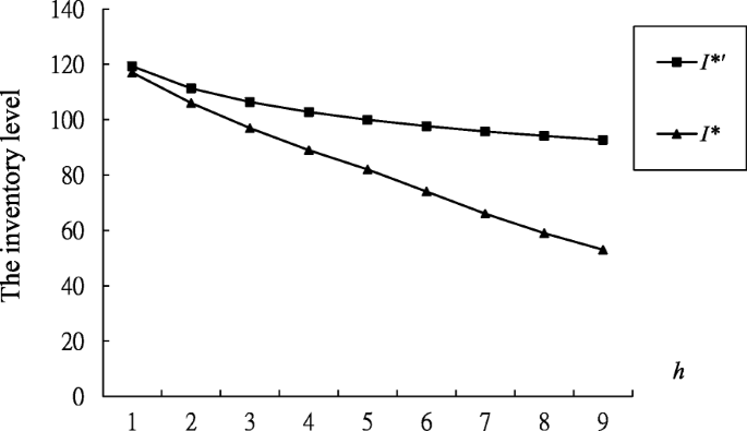
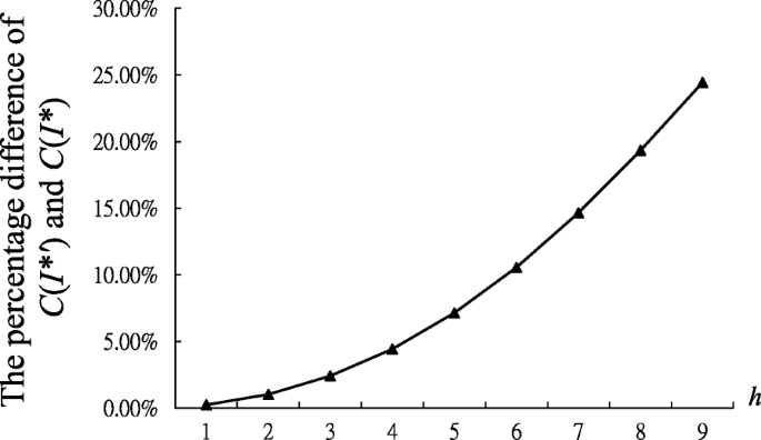
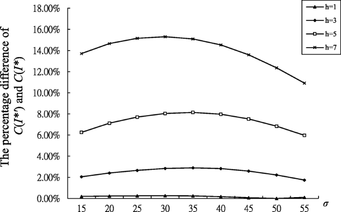
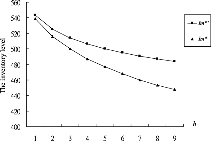
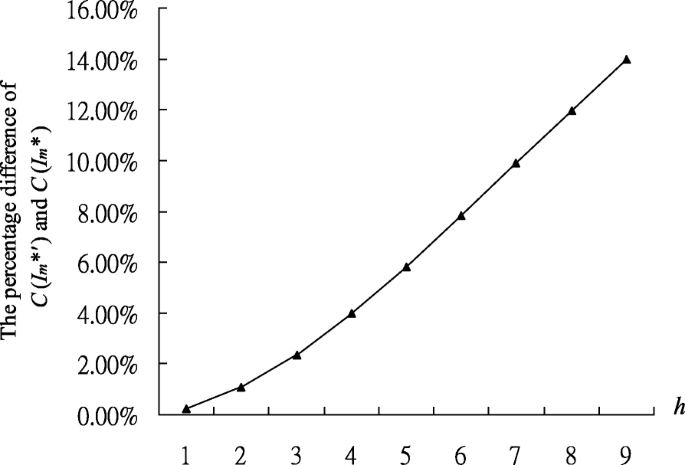
The single-period model is studied first. Note that in (3.3) the second-order derivative of the objective function in Program P2 is greater than 0, and thus the objective function is convex. To get the optimal solution of Program P2 (I^∗), we just find the value of I that make C^′(I) in (3.2) equal 0 with numerical experiments. Figures 3 and 4 examine the differences of I^∗ andI^∗′ as well as C(I^∗) and C(I^∗′) respectively when we change the unit holding cost h from 1 to 9 and keep all the other parameters constant. In Fig. 3, I^∗ is always less than I^∗′, which is consistent with Theorem 1. It also shows that the difference between I^∗′ and I^∗ increases as the unit holding cost increases. It can be explained as follows. As the unit holding cost increases, both I^∗′ and I^∗ decrease (Theorem 2), and the scenario in Fig. 2 will have a greater chance to occur. Then the inventory cost for consumed products weighs more in the cost function. Since the deviation between I^∗′and I^∗ is mainly caused by this term, the difference tends to increase with the unit holding cost. Figure 4 shows that the percentage difference of C(I^∗′) and C(I^∗), i.e.,[C(I^∗′) − C(I^∗)]/C(I^∗), increases as the unit holding cost increases. Figure 4 is consistent with Fig. 3, which shows that as the unit holding cost increases, the scenario in Fig. 2 will have more of a chance to occur and the inventory cost for consumed products in the cost function plays a more important role. In Figs. 3 and 4, with a low unit holding cost, the difference of the cases with and without the consumed inventory cost in the objective function, in terms of the inventory level and expected average inventory cost, is not significant. In such a scenario, I^∗′ does not deviate from I^∗ much and is a good approximation of I^∗ for it has the analytical form expressed in (3.1). It can greatly facilitate the analysis of more complicated situations. However, we can also observe in Figs. 3 and 4 that when the unit holding cost is relatively high, the deviation of I^∗′ from I^∗ becomes non-ignorable. In this situation, I^∗′ is not suitable as the approximation of I^∗ otherwise it can cause the expected average cost C(I^∗′) to deflect from the actual minimum expected inventory cost C(I^∗) significantly. Numerical experiments may help in such a situation to derive the optimal inventory level as well as the minimum inventory cost. In Fig. 5, let the standard deviation of the demand distribution vary under different unit holding costs, and fix the values of all the other parameters. It shows that with a higher unit holding cost, the volatility of the demand has an upward bending relation with the percentage difference of C(I^∗′) and C(I^∗). In contrast, with a lower unit holding cost, the impact of the demand volatility on this percentage is much lower or even ignorable. The insensitivity of the percentage difference to the demand variation for a low unit holding cost also demonstrates that I^∗′ is a suitable approximation of I^∗ in such situations. The inverse U-shape of the curves in Fig. 5 can be explained as follows. Note that the difference between I^∗ and I^∗′ is mainly determined by the fourth term in Program P2. When the degree of demand uncertainty is low, the first, second and fourth terms in P2are relatively small, compared to the third term. In this situation, the small weight of the fourth term in the total cost function only leads to a small difference between I^∗ and I^∗′. Consequently, the percentage cost difference is also small. Then the percentage cost difference initially increases as the degree of demand uncertainty increases from a very low level. When the degree of demand uncertainty goes beyond a certain high level, the weight of overstocking and understocking costs, i.e., the first two terms in P2, tend to be larger. Then the fourth term in P2 in this situation tends to be less important in the cost function. It leads to smaller differences between I^∗ and I^∗′ and lower percentage cost differences.

Fig. 3

The inventory level vs. the unit holding cost for the model with instantaneous receipt

Fig. 4

The percentage difference of C(I^∗′) and C(I^∗) vs. the unit holding cost for the model with instantaneous receipt

Fig. 5

The percentage difference of C(I^∗′) and C(I^∗) vs. the standard deviation of the demand distribution under different unit holding costs for the model with instantaneous receipt

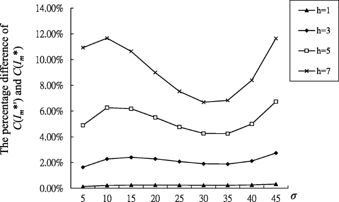
Next we examine the model without instantaneous receipt. Due to the form of the objective function in Program P4, we cannot derive the closed-form optimal solution. Thus we first conduct numerical experiments to get the optimal solution of Program P4, and examine the impacts of factors on the differences of ${I}_m^{\ast }$ and ${I_m^{\ast}}^{\prime }$ as well as ${C}_m\left({I}_m^{\ast}\right)$ and ${C}_m\left({I_m^{\ast}}^{\prime}\right)$ respectively. In general, numerical results for the model without instantaneous receipt are similar to those with instantaneous receipt. More specifically, Figs. 6 and 7 reveal similar patterns to Figs. 3 and 4, respectively. In Figs. 6 and 7, with a low unit inventory holding cost, the deviations of the cases with and without the consumed inventory cost considered in the objective function, in terms of the inventory level and expected average inventory cost, are trivial, while they are noteworthy with a high unit holding cost. In Fig. 8, let the standard deviation of the demand distribution vary under different unit holding costs, with other things constant. It shows some interesting patterns that cannot be revealed by examining the objective function of Program P4. A group of wave curves under different unit holding costs are graphed in this figure, and the amplitude of fluctuation increases as the unit holding cost increases. It indicates that the demand uncertainty has alternate positive and negative impacts on the difference of ${C}_m\left({I}_m^{\ast}\right)$ and ${C}_m\left({I_m^{\ast}}^{\prime}\right)$ in the model without instantaneous receipt.

Fig. 6

The inventory level vs. the unit holding cost for the model without instantaneous receipt

Fig. 7

The percentage difference of C(I^∗′_m) and C(I^∗_m) vs. the unit holding cost for the model without instantaneous receipt

Fig. 8

The percentage difference of C(I^∗′_m) and C(I^∗_m) vs. the standard deviation of the demand distribution under different unit holding costs for the model without instantaneous receipt

Moreover, to exam whether above results are robust, we have further conducted.

In numerical experiments for different values of $\frac{\pi }{h+\pi }$, the shapes of curves are very close to the above results.

Our numerical experiments show that there exist differences in optimal inventory levels with and without the holding cost for consumed stock in the total cost function. A suboptimal solution is obtained if the cost for consumed stock is excluded in the cost function when making decisions. The numerical experiments indicate that this inventory level difference and associated total cost difference increase as the unit holding cost increases and can be affected by the degree of demand uncertainty. These findings provide some useful insights for practitioners. When the unit holding cost is relatively high compared to the unit backordering cost, there is more chance to have understock at the end of the period. That is, the scenario in Fig. 2 will have a greater chance to happen. In this situation, the decision on inventory level will remarkably affect the holding cost for consumed items. Our analysis shows that the inventory level considering the holding cost for consumed stock will be lower than the one determined by the model further taking into account such holding costs. In other words, the former one is inferior to the latter one when the total inventory cost function includes understocking costs, overstocking costs and holding costs for consumed stock. The difference in the inventory levels will lead to associated cost differences. Such cost difference also increases with the unit holding cost, and can be affected by the degree of demand uncertainty. Since the unit inventory holding cost usually covers storage space costs, handling and service costs, risk costs and capital costs, one or more such factors may cause a high unit holding cost. For example, luxury products or products requiring specific storage conditions may have a high unit holding cost. When inventory decisions are made for these products, the holding cost for consumed items should be included in the total cost function to obtain the optimal inventory level. Otherwise, a suboptimal solution will be obtained.

Conclusion

In this work, we revisit the newsvendor model by considering the consumed stock holding cost in the cost function. In the classic model, we assume the inventory level has no impact on the holding cost for consumed stock during one period, where the average holding cost for this portion of inventory is usually approximated as half the product of the unit holding cost and the expectation of the demand in that period. It works when the ratio of unit holding cost to the unit shortage cost is low. However, without this condition, the approximation can deviate significantly from the actual expected cost. The higher unit holding cost can be attributed to the high capital cost, insurance cost, holding cost for specific storage conditions, and, more prominently, coming carbon charges. With today’s trends of price-based policies for reduction of greenhouse gas emissions, as well as the advance of technologies in warehouse management, holding costs have been rising significantly in some industries. To mitigate the potential shortcomings of the classic model, we add the holding cost for consumed inventory into the cost function. The models with and without instantaneous receipt are formulated and analyzed.

For the model with instantaneous receipt, analysis shows that the optimal inventory level is lower if the consumed inventory cost is considered in the cost function, other things being constant. The relationships between the optimal inventory level and the unit holding cost as well as the unit backordering cost are shown. Numerical experiments are conducted to examine the factors that affect this deviation. Other things being constant, the deviation increases as the unit inventory holding cost increases, for both models. The uncertainty of demand, which is measured by its standard deviation, has either positive or negative impacts on the deviation depending on the specific circumstance. Both analyses and numerical experiments indicate the deviation caused by ignoring the holding cost for consumed inventory is unacceptable in some circumstances. The approximation, i.e., half the product of the unit holding cost and the expectation of the demand in the period, can lead to the closed-form expression of optimal inventory level (or position) and facilitate analyses of more complicated problems. In such situations, well-designed numerical experiments and simulations should be employed to conduct further research.

References

Arrow, K. J., Harris, T., & Marschak, J. (1951). Optimal inventory policy. Econometrica, 19(3), 250–272.
Arrow, K. J., & Karlin, S. (1958a). Smoothed production plans. In K. J. Arrow, S. Karlin, & H. Scarf (Eds.), Studies in the Mathematical Theory of Inventory and Production (pp. 61–69). Stanford: Stanford University Press.
Arrow, K. J., & Karlin, S. (1958b). Smoothed production plans. In K. J. Arrow, S. Karlin, & H. Scarf (Eds.), Studies in the Mathematical Theory of Inventory and Production (pp. 70–85). Stanford: Stanford University Press.
Berling, P. (2008). The capital cost of holding inventory with stochastically mean-reverting purchase price. European Journal of Operational Research, 16(2), 620–636.
Correia, I., Melo, T., & Saldanha-da-Gama, F. (2013). Comparing classical performance measures for a multi-period, two-echelon supply chain network design problem with sizing decisions. Computers & Industrial Engineering, 64(1), 366–380.
Erlebacher, S. J. (2000). Optimal and heuristic solutions for the multi-item newsvendor problem with a single capacity constraint. Production and Operations Management, 9(3), 303–318.
Evans, R. V. (1967). Inventory control of a multiproduct system with a limited production resource. Naval Research Logistics Quarterly, 14(2), 173–184.
Ferguson, M., Jayaraman, V., & Souza, G. C. (2007). Note: An application of the EOQ model with nonlinear holding cost to inventory management of perishables. European Journal of Operational Research, 180(1), 485–490.
Hadley, G., & Whitin, T. M. (1963). G. Analysis of Inventory Systems. Englewood Cliffs: Prentice-Hall.
Heyman, D. P., & Sobel, M. J. (1984). Stochastic models in operations research (Vol. Vol. II). New York: McGraw-Hill.
Krishnan, H., & Winter, R. A. (2010). Inventory dynamics and supply chain coordination. Management Science, 56(1), 141–147.
Li, S., & Lin, B. (2006). Accessing information sharing and information quality in supply chain management. Decision Support Systems, 42(3), 1641–1656.
Mieghem, J. A. V. (2007). Risk mitigation in newsvendor networks: Resource diversification, flexibility, sharing, and hedging. Management Science, 53(8), 1269–1288.
Olivares, M., Terwiesch, C., & Cassorla, L. (2008). Structural estimation of the newsvendor model: An application to reserving operating room time. Management Science, 54(1), 41–57.
Petruzzi, N. C., Wee, K. E., & Dada, M. (2009). The newsvendor model with consumer search costs. Production and Operations Management, 18(6), 693–704.
Porteus, E. L. (1971). On the optimality of generalized (s, S) policies. Management Science, 17(7), 411–426.
Porteus, E. L. (1972). The optimality of generalized (s, S) policies under uniform demand densities. Management Science, 18(11), 644–646.
Porteus, E. L. (1990). Stochastic inventory theory. In D. P. Heyman & M. J. Sobel (Eds.). North Holland: Elsevier Science Publishers.
Shi, M., & Yan, X. (2017). Heterogeneous consumers, search and retail formats. Frontiers of Business Research in China, 11(4), 525–544.
Veinott, A. F. (1965a). Computing optimal (s, S) inventory policies. Management Science, 11(5), 525–552.
Veinott, A. F. (1965b). Optimal policy for a multi-product, dynamic, non-stationary inventory problem. Management Science, 12(3), 206–222.
Acknowledgements
The research is partially supported by Natural Science Foundation of Guangdong (2015A030313823), Zhuhai Outstanding Discipline Project-Accounting and UIC college research grant.
Author information
Authors and Affiliations
Contributions
ST carried out models setup and analysis; SC helped draft the manuscript and made the figures in the draft; JWW helped conduct the literature review and drafted the manuscript; HY helped construct models and conducted numerical experiments. All four authors read and approved the final manuscript.
Corresponding author
Ethics declarations
Competing interests
The authors declare that they have no competing interests.
Publisher’s Note
Springer Nature remains neutral with regard to jurisdictional claims in published maps and institutional affiliations.
Rights and permissions
Open Access This article is distributed under the terms of the Creative Commons Attribution 4.0 International License (http://creativecommons.org/licenses/by/4.0/), which permits unrestricted use, distribution, and reproduction in any medium, provided you give appropriate credit to the original author(s) and the source, provide a link to the Creative Commons license, and indicate if changes were made.
About this article
Cite this article
Tang, S., Cho, S., Wang, J.W. et al. The newsvendor model revisited: the impacts of high unit holding costs on the accuracy of the classic model. Front. Bus. Res. China 12, 12 (2018). https://doi.org/10.1186/s11782-018-0034-x
Received:
Accepted:
Published:
DOI: https://doi.org/10.1186/s11782-018-0034-x